Software
Introduction
Since we started this project, we realized how difficult it was to get a Quartz Crystal Microbalance, although more than difficult, it was expensive. Once we got deeper into the research, our goal was only one: to give other people the possibility to get information from their Quartz Crystal Balance in a simple and efficient way.
So, our software is a user-friendly interface that takes the user by the hand, step by step, and also gives the possibility to adapt the experiments to different scenarios for different needs.
The developed software is so flexible that the idea is that it can be used in other QCMs, not necessarily the one developed by us. We realized that the software used by commercial microbalances was only provided once you purchased their product.
urthermore, modifying it would not be an easy task, and its use would be limited only to the company that sold it to you. Our philosophy was always to develop free software, with detailed indications within the code so that it can be modified, and above all, that it adapts to different needs.
Final Product
Download files
The link on Gituhub is provided so that anyone can download the necessary files:
Application folder
Or if you prefer to download directly, a folder is for the application:
Support files
Files like the Arduino software, Teensyduino, its libraries, among others are presented below:
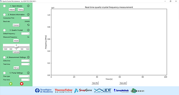
The Interface is as follows (Figure 1).
How to install it?
First, access the Github link previously shown and download the folder. Once you unzip it, you must run the program with ".exe" ending. Accept all permissions and select the location where you want to install it. A new folder is created, when you open it you will find the software called "QCM by iGEM TEC CEM 2021", it is of the "Application" file type. This file is opened and the interface is ready. Below is a tutorial to get it.
Add-on's installation
The interface works with the help of other applications, mainly Arduino. This is because it offers the possibility of assembling circuits and obtaining information from sensors with a fairly intuitive programming language. For this reason, the first thing to do is to install the Arduino software, the version used is 1.8.16. It is recommended to install the program directly in the "Program Files" folder located on the local disk. This and the following files are located in the previously mentioned folder under support files. In case you are working with Teensy, the Teensyduino application is also installed. Finally, the libraries needed to upload the program to the microcontroller.
Step by Step
In the previous video, we showed how to obtain the measurements and their respective graph and text file, but in this section we will go more in depth about each section.
1. Open Arduino
First step of the software is to select which microcontroller you are using (Figure 2). Before pressing one of the buttons, be sure to complete the following steps:

Figure 2. Open Arduino step. Select the microcontroller you are working with.
1.1- Install the Arduino software, the one used is version 1.8.16 (Figure 2). You can find this program in the folder called 'QCM support files'. Unzip the folder and run the 'arduino' application. It is also important to set Arduino as the default application to open files ending in '.ino'. A quick way to do it is to save an empty Arduino file to the desktop, select the properties option by right-clicking, locate the option 'opens with', select 'change', then 'find another application on the computer', and select the arduino app in the downloaded folder.

Figure 3. Arduino software.
1.2- From the same folder called 'QCM support files', go to 'Libraries' and download 'FreqCount', and 'AD9833'. Then, in Arduino select Program> Include library> Add ZIP library, and then select each of the aforementioned folders (Figure 4).

Figure 4. Libraries to import
1.3- If you are using an Arduino as a microcontroller, you can continue to step 4. It is important to mention that the Arduino is used for quartz crystals less than 5 MHz, if your measurement is greater, for example 10 MHz, you will have to use a Teensy. For the latter case, you must install the program that makes it compatible with the Arduino interface, which is called Teensyduino. In the same way, you can find it in the 'Libraries' subfolder.

Figure 5. Install Teensyduino
1.4- Now, it is time to select the 'Tools' tab in Arduino software. Select the board you are using, for example Teensy 4.1 or Arduino Nano. Then choose the port it is connected to. Finally, use the buttons on the Arduino interface to verify the program and upload it (Figure 6).
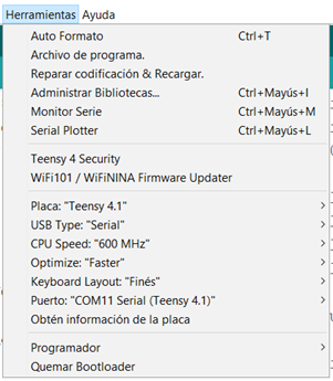
Figure 6. Example of connection of al Teensy 4.1
2. Arduino Information
The second step is simpler, you only have to select the port to which your device was connected and press the 'Connect' button. You probably won't see the available port until you upload the Arduino program, so once you've done that, hit the refresh button and now you'll have the option. If the port is not available or is the wrong one, make sure you have the usb cable connected correctly, you could also try to disconnect other inputs that are time, even having Bluetooth turned on in your computer could show devices that you do not want to see .
The communication speed with the Arduino is also shown, which is in bits per second. A relatively high value was chosen for proper communication and more accurate real-time values. This section is used to mention the importance of properly following the sequence of steps, if it is not done in this way, there is some missing data or it was not connected properly, a circle on the left will be shown in orange, check the information entered. If everything was done correctly, a green circle will light up, which means that you can proceed to the next section.
3. Quartz Crystal
At this point, the frequency established by the manufacturer must be selected, 4, 5, and 10 MHz are given as options, since they are the most used in quartz crystal microbalances, but others can be added with simple changes in the code. Below this data, the frequency measured at that moment is shown. It is here where Hardware and Software become one, since the quartz crystal microbalance "must be assembled and connected correctly so that the software begins to graph the data acquired in real time. A great advantage of this application is that it can be used for any QCM, even commercial ones.
Then, there is one of the most useful tools that we designed, which is the option of calibrating the frequency, that is, increasing or decreasing the value of the selected crystal. The idea of this is that the user manages to resonate the crystal by applying the exact frequency of this between its terminals. This was implemented because the frequency set by the manufacturer has a certain tolerance, which means that it may be slightly above or below the value provided. The resonance can be appreciated because there is a notable decrease in said value and the variations due to any event near the crystal are significant .
4. Measurements Settings
It is time to configure the measurements to be obtained from the quartz crystal. The options you choose depend on the experiment that is being carried out. The first thing is to select the time difference between each of the measurements. Initially, a measurement of the output frequency of the quartz crystal is made in 1 second. There are several options to select the one that best suits each case. Then, the total time of the experiment is selected. It is the amount of information that will be shown on the graph and that which can be saved. It is recommended to be conservative with this value and choose times higher than the assumptions, this in order to have more information, instead of less
5. Pump Settings
The last step is to select the type of flow that you want to use and the operating time. You have the following options:
-
Manual. This is very useful, since it allows the user to carry out the measurement directly by himself, the micropipetting technique can be used, which opens up a large number of possible experiments to be carried out. For this case, the selected flow time does not matter, as none of the pumps will be activated.
-
Go-no-Go, this option and the next is for liquid biosensing. This name refers to activating the inlet pump for a certain time, then leaving the fluid in the chamber in contact with the quartz crystal for another amount of time, and finally activating the outlet pump to remove the fluid. It is an excellent option to compare the behavior of a fluid and its adhesion with respect to time with a biofilm placed on the crystal. In this case, the selected flow time will indicate the time that the first pump will last on, the same time for the time inside the chamber, and in the same way for the time of the outlet pump.
-
Continuous. In this option, both pumps are turned on at the same time, so that everything that goes in comes out, this process is almost immediate, an excellent affinity between the analyte and the biofilm is needed to achieve that the changes in frequency can be appreciated. The selected time indicates how long both pumps will be working. The play button starts the experiment, the stop button restarts the measured values. If you want to make a new measurement, you must press stop and play again. Once all the data has been plotted, it is possible to download the acquired information in txt format for later analysis, as well as the graph with 'Save file' and 'Save plot' buttons, respectively.
Codes
Arduino Code
There are some differences between the Teensy and the Arduino files, in terms of the pins used, and the numerical value that a function takes. However, the same logic is followed. The program starts by importing libraries, then defining the type of variables and assigning their respective values. Then the void setup is configured, where initial conditions are defined such as the communication speed, the initial configuration of the signal generator (A9833), and the motor pins as output.
Then, it is important to mention how the Arduino and Python alliance works. It happens that there is information that must be sent from Arduino to Python, such as the output frequency reading of the quartz crystal. And also inversely, from Python to Arduino, when the crystal is selected, the calibration is done, or the type of flow and the on time of the pumps is selected. For this reason, we chose to label the data in a certain way so that the programs decode it correctly. The label "mot" sends the frequency data requested in Python, "del" gives the time delta between each measurement, "flo" the type of flow and its respective time, and "add" the measured frequency, which will be the one to be plotted.
A complex part of the programming was the pumps. These worked correctly in isolation, but when they were implemented in the code, the code failed to measure the frequency in real time, it had slight lags. This was mainly due to the delays that were necessary to indicate the time they should operate. This could have been solved quickly and efficiently using threads, but in Arduino they are not used directly, more or less. What is commonly used is the function "millis()" which measures the execution time of the program, that is, since it was uploaded to the board. This has the advantage of being able to make functions dependent on this time, i.e. to start executing 10 seconds after the program has been started, for example. But in our case, the time depends on the user, so we had to properly handle this function, in simple terms, the solution was to have two timers, which start at the same time, but one of them is stopped when the indication to turn on the pumps and the type of flow is sent from Python. This value is subtracted from the one that continues counting, and now a conditional is set so that the Arduino turns on the pumps while the time difference is less than the pumping time requested by the user.
Python Code
Now it is turn to describe Python code. However, in this case the amount of work was greater, to be exact, 1251 lines of code were written, so describing it completely is not so simple. However, quite descriptive comments were made throughout the text, because as we mentioned, we hope that our software will be as useful to other teams as it was for us in our measurements, we really managed to make it easier for ourselves to obtain information. In the same way, it is expected that the people who require the code implement it to their taste and needs, making all the modifications that they consider.
Again, from top to bottom, we start importing libraries, followed by the definition of variables, and start declaring functions. The most important ones and the main challenges of this software development are mentioned. First, the communication between python and arduino, which is serial, had to be established. This function was much to investigate, with which it was found that there was already a library to connect to Arduino by declaring the port and the baud rate of communication. The next challenge was to get the sensor values and other indications from the Arduino.
As mentioned above, the proposed solution was to communicate via tags, which prevents incorrect information from being read. So the next steps consisted of handling arrays. In that same function, the problem was to be able to plot the results in real time, basically an empty array was made which was loaded as each of the data arrived, and with an iteration counter, the x-axis was filled. These iterations were changed to time values, by the factor selected by the user. It was necessary to create a thread to obtain reliable data acquisition, i.e. not affected by other processes. In addition, displaying the graph in real time required a lot of support in forums to work with matplot and canvas. Finally, there is everything related to the graphic interface, for which specialized libraries were needed.